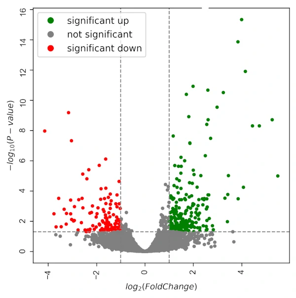
DeSeq2 is a popular R package for analyzing RNA-seq count data. It can be used to identify differentially expressed genes between two or more experimental groups. In this tutorial, I’ll walk you through the basic steps of using DeSeq2 to perform a differential expression analysis.

Install

Before we begin, you’ll need to make sure that you have R and the DeSeq2 package installed on your system. You can install R from the official website (https://www.r-project.org/), and install the DeSeq2 package by running the following command in your R console:

install.packages("DeSeq2")

Once you have R and the DeSeq2 package installed, you can start by loading the package:

library(DeSeq2)

Let’s begin

The first step in using DeSeq2 is to import your RNA-seq count data into R. DeSeq2 expects your data to be in the form of a matrix, where rows represent genes and columns represent samples. Each cell in the matrix should contain the count of reads for a particular gene in a particular sample. Your data should also include a column called “condition” that specifies the experimental group that each sample belongs to. Here is an example of how you can import your data into R:

data <- read.table("rnaseq_data.txt", sep="\t", header=TRUE)

Once you have imported your data, you can use the DeSeqDataSetFromMatrix function to convert it into a DeSeqDataSet object that can be used by DeSeq2:

dds <- DeSeqDataSetFromMatrix(countData = data, colData = data[,c("condition")], design = ~ condition)

In this example, countData parameter is the matrix of count data, colData parameter is the condition column, and design parameter is a formula that specifies the experimental design.

Once you have created the DeSeqDataSet object, you can use the estimateSizeFactors function to estimate size factors for your samples. Size factors are used to account for differences in sequencing depth across samples:

dds <- estimateSizeFactors(dds)

Once you have estimated the size factors, you can use the estimateDispersions function to estimate the dispersion of the counts for each gene. Dispersion is a measure of how much the counts for a gene vary across samples:

dds <- estimateDispersions(dds)

Now that you have estimated the size factors and dispersions, you can use the nbinomTest function to perform a likelihood ratio test for differential expression. The nbinomTest function compares the likelihood of the observed count data under the null hypothesis (i.e., that there is no difference in expression between the two groups) to the likelihood of the data under the alternative hypothesis (i.e., that there is a difference in expression). The function returns a DeSeqResult object that contains the test results:

res <- nbinomTest(dds, "conditionA", "conditionB")

conditionA and conditionB are the two experimental groups you are comparing, you can replace them with your own group labels.

Finally, you can use the results function to extract the results from the DeSeqResult